Articles

Karpathy's Software 3.0 Playbook
Twelve lessons from Andrej Karpathy's Sequoia interview: Software 3.0, vibe coding versus agentic engineering, jagged intelligence, and why December 2024 was the inflection most people missed.
Commentary 10 min AIAI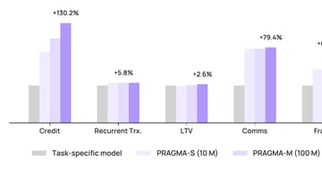
Inside PRAGMA: Revolut's Foundation Model for Banking
Revolut's PRAGMA is a 1B-parameter encoder trained on 24B banking events. Reading the paper, comparing with Nubank's nuFormer, planning a rebuild.
Analysis 6 min AIAI
The Moral Philosophy of Investing in Ignorance
Constraint arbitrage, the sidecar problem, and who bears the distributional cost of investing under ignorance. The final installment of Edge of Knowledge.
Analysis 8 min Quantitative FinanceQuant
Bet Sizing at the Frontier
The Kelly Criterion assumes you know your probability of winning. In a UU world, you don't, and heuristics like Zeckhauser's Maxim B replace false precision.
Analysis 9 min Quantitative FinanceQuant
The Geometry of Who Knows What
When neither side can define the states of the world, adverse selection fears are misplaced. Zeckhauser's information matrices and constraint arbitrage.
Analysis 9 min Quantitative FinanceQuant
Do Not Disturb My Circles
AlphaFold cost under $1M to train. OpenAI spends $2.3B on inference. The chatbot era consumed the talent and compute that could have cured diseases.
Commentary 13 min AIAI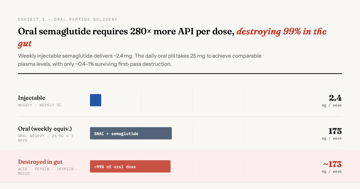
Why Lilly's Weight Loss Pill Isn't a Peptide
Oral semaglutide destroys 99% of its active ingredient per dose. Lilly's Foundayo skips the problem entirely. Inside the $70B oral GLP-1 pill race.
Analysis 9 min MedicineMedicine
Ambiguity by Design
Ellsberg proved people flee unknown odds. Zeckhauser showed their flight creates mispricing. Part 2 on ambiguity aversion, comparative ignorance, and investing.
Analysis 8 min Quantitative FinanceQuant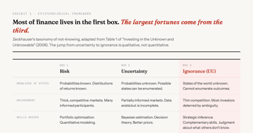
Three Kinds of Not-Knowing
Knightian uncertainty splits not-knowing into risk, uncertainty, and ignorance. A century after Knight and Keynes, most of investing still ignores the split.
Analysis 9 min Quantitative FinanceQuant
On-Device AI Models Will Be The New Reason to Upgrade Your Phone
Smartphones haven't had a compelling upgrade story in years. On-device AI models, distilled from frontier systems like Gemini, are about to change that. Parameters are the new megapixels.
Commentary 5 min AIAI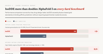
AI Can Now Design Drugs in Seconds; We Still Can't Tell You If They Work.
IsoDDE doubles AlphaFold 3 on hard benchmarks and beats physics-based gold standards. But no AI drug has FDA approval. What $4B in pharma deals actually mean.
Essay 6 min MedicineMedicine
The Last Architecture Designed by Hand
The transformer's limits are now mathematical proofs, not empirical hunches. Hybrids are in production. AI is searching for its own replacement. Here's what comes after.
Analysis 6 min AIAI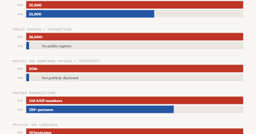
MCP vs A2A in 2026: How the AI Protocol War Ends
MCP leads with 97M monthly SDK downloads and 10,000+ servers. A2A fills a different layer. Analysis of the agentic AI standards war with historical parallels.
Analysis 8 min AIAI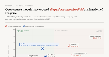
AI Models Are the New Rebar
Qwen 3.5-35B runs on a gaming PC and matches Claude Sonnet 4.5. When the commodity version is 95% as good and 97% cheaper, you have a pricing problem.
Analysis 7 min AIAI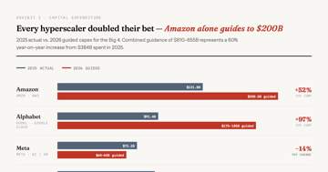
AI Capex Arms Race: Who Blinks First?
Alphabet's free cash flow is on track to fall 90% in 2026. Amazon's is at $11B. $690B in AI capex is cannibalizing the cash that justified these valuations.
Analysis 8 min InvestingInvesting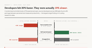
93% of Developers Use AI Coding Tools. Productivity Hasn't Moved.
METR found experienced developers 19% slower with AI, despite feeling 20% faster. At 92.6% adoption, organizational productivity gains remain roughly 10%.
Analysis 9 min TechTech
Peter Thiel's Physics Department
Peter Thiel says physics stalled in 1972. Then GPT-5.2 proved a new result in theoretical physics. The 75:1 AI compute gap between commerce and science.
Essay 8 min AIAI
When AI Labs Become Defense Contractors
The Anthropic-Pentagon standoff isn't an ethics story. It's a replay of the 1993 Last Supper that consolidated 51 defense primes into 5, at Silicon Valley speed.
Analysis 8 min AIAI
Every Bulge Bracket Bank Agrees on AI
I read 12 AI research reports from Goldman Sachs, JPMorgan, UBS, and 6 other banks. Here's the consensus they're pushing, and what they're not saying.
Analysis 10 min AIAI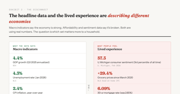
People Live in Levels, Not Rates
Prices rose 25% since 2020 and won't come back. The levels-vs-rates problem explains the vibecession, the Stewart-Thaler debate, and why nobody trusts economists.
Commentary 7 min MacroMacro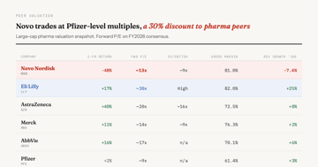
Novo Was Europe's Most Valuable Company
Novo Nordisk lost 75% since June 2024. CagriSema failed vs Zepbound, US pricing is resetting lower, and Lilly leads on every axis. Full breakdown with numbers.
Analysis 10 min MedicineMedicine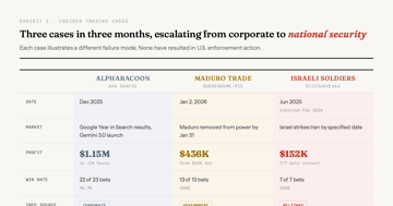
The Absolute Insider Mess of Prediction Markets
A Google insider made $1.15M on Polymarket in 24 hours. Israeli soldiers bet classified strike timing. Why prediction markets need insider trading regulation.
Analysis 11 min InvestingInvesting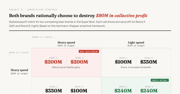
Economics of a Super Bowl Ad
A 30-second Super Bowl spot costs $8M. The real price is $16–23M. The ROI evidence is mixed. A deep look at the pricing, the prisoner's dilemma, and the NFL.
Analysis 11 min EconomicsEconomics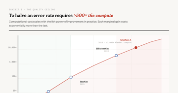
The Impossible Backhand
AI converges to the mean by design. Ninth-power scaling costs and a 53-point gap on Humanity's Last Exam show domain expertise is appreciating, not declining.
Essay 10 min AIAI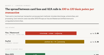
Europe's $24 Trillion Payment Breakup Is Really a Bet on Infrastructure Arbitrage
The EuroPA alliance connected 130 million users across 13 countries overnight. But this isn't really about sovereignty. It's an infrastructure arbitrage exploiting a 100-120bps spread between card network fees and SEPA Instant rails, accidentally protected by the EU's own regulation.
Essay 14 min MacroMacro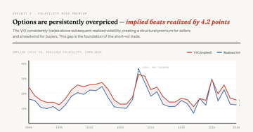
Long Volatility Premium
One River's data shows beta-adjusted long volatility outperformed the S&P 500 over 40 years. Goldman, AQR, and Universa agree on the mechanism but disagree on implementation. A synthesis of the evidence.
Essay 12 min Quantitative FinanceQuant
The SaaSpocalypse Paradox
AI capex failure and AI replacing all software are mutually exclusive. Why the 2026 SaaSpocalypse is a $2 trillion pricing error, not an extinction event.
Essay 8 min AIAI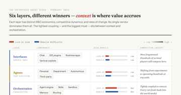
Don't Go Monolithic; The Agent Stack Is Stratifying
The enterprise AI agent stack is stratifying into six layers with different winners at each. Models commoditize; context — your organizational world model — compounds. A framework for agentic AI architecture decisions.
Essay 8 min AIAI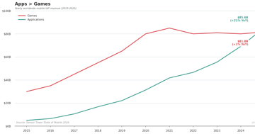
Where Mobile Money Goes Now
Apps overtook games in mobile IAP revenue for the first time in 2025, driven by $3.5B in GenAI growth. Analysis of Sensor Tower's State of Mobile 2026 report.
Analysis 3 min AIAI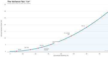
Variance Tax
Variance drain is the hidden cost of volatility: why a portfolio averaging +10% can lose money. The ½σ² formula explains the gap between paper and real returns.
Essay 4 min Quantitative FinanceQuant
Claude Opus 4.6: Anthropic's New Flagship AI Model for Agentic Coding
Claude Opus 4.6 brings a 1M token context window, 68.8% ARC-AGI-2, and Agent Teams to Claude Code. Full benchmark comparison vs GPT-5.2 and Gemini 3 Pro with pricing analysis.
Commentary 6 min AIAI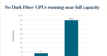
Buying the Haystack Might Not Work This Year
a16z sees AI fundamentals thriving with 80% GPU utilization. AQR sees the CAPE at the 96th percentile. Both have data. Both may be right.
Commentary 4 min AIAI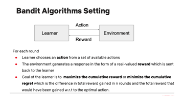
Bandits and Agents: Netflix and Spotify Recommender Stacks in 2026
How hybrid recommender systems balance multi-armed bandits against LLM inference cost economics in 2026. A deep dive into Netflix recommendation algorithm architecture and Spotify's AI DJ recommender system.
Essay 5 min AIAI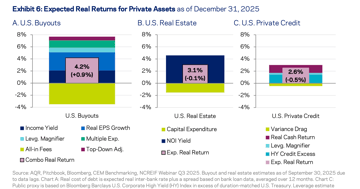
Is Private Equity Just Beta With a Lockup?
AQR's 2026 data shows private equity returning 4.2% versus 3.9% for public equities. The 30bp illiquidity premium barely justifies years of lockup.
Commentary 4 min Quantitative FinanceQuant
Britain's Strategic Limbo
Britain faces strategic isolation: locked out of EU defense cooperation, unwilling to join Trump's coalition. The mid-Atlantic bridge has nowhere to land.
Analysis 3 min MacroMacro
The Rise of Middle Power Realism
At Davos 2026, Carney told allies to take down the signs of the liberal order. Middle powers are learning to navigate between giants without illusions.
Analysis 4 min MacroMacro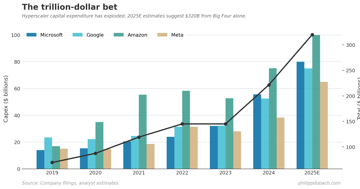
The Most Expensive Assumption in AI
Sara Hooker's research challenges the trillion-dollar scaling thesis. Compact models now outperform massive ones as diminishing returns hit AI.
Commentary 4 min AIAI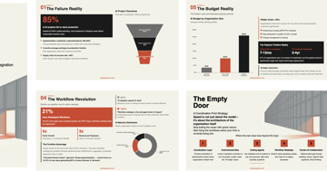
Enterprise AI Strategy is Backwards
85% of AI projects fail. Only 26% translate pilots to production. The winners automate the coordination layer where employees spend 57% of their workday.
Essay 2 min AIAI
Big in Japan
Japan holds $5 trillion in foreign assets. With 30-year JGB yields now above 3%, the carry trade that defined Japanese investing faces new friction.
Commentary 2 min MacroMacro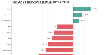
Ozempic is Reshaping the Fast Food Industry
Cornell research: GLP-1 users cut grocery spending 5.3%, fast food 8%. With 16% household adoption and savory snacks down 10%, food stocks face headwinds.
Commentary 4 min MedicineMedicine
Does AI mean the demand on labor goes up?
AI was supposed to free us. The Jevons paradox plays out in real time: efficiency expands workload, not leisure. 77% of workers say AI added to their work.
Commentary 2 min AIAI
Repo might be even bigger than we thought
New OFR data reveals $12.6 trillion in daily repo exposures—$700 billion larger than previous estimates. The plumbing of modern money remains poorly understood.
Commentary 5 min MacroMacro
The Market Can Stay Irrational Longer Than You Can Stay Solvent
Steve Eisman explains how U.S. equity markets have structurally decoupled from everyday economic reality through concentration and passive investing.
Commentary 4 min InvestingInvesting
Beyond Vector Search: Why LLMs Need Episodic Memory
Context windows aren't memory. Explore EM-LLM's episodic architecture, knowledge graph tools like Mem0 and Letta, and why vectors fail for sequential data.
Essay 3 min AIAI
Praise by Name, Criticize by Category: Warren Buffett Retires at 95
Buffett exits after paying $26.8B in taxes. What 60 years of letters reveal about admitting mistakes, insurance float, and why Abel inherits $300B in cash.
Essay 5 min InvestingInvesting
Apple's AI Bet: Playing the Long Game or Missing the Moment?
Apple's $157B cash pile and Gemini-powered Siri shift show a restrained AI strategy. Analysis of whether Apple wins as AI models become commodities.
Commentary 3 min AIAI
How AI is Shaping My Investment Portfolio for 2026
Rebalancing for 2026: reducing S&P 500 at 40× CAPE, adding Europe after Germany's €1T pivot, and bonds at 4.2% yields. Full allocation rationale.
Essay 10 min InvestingInvesting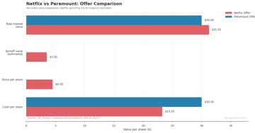
Not Logan Roy: Netflix vs. Paramount's Bidding War
Netflix's $72B Warner Bros deal vs Paramount's hostile $30/share tender. Deal mechanics, aggregation theory, and why internet distributors win streaming.
Analysis 7 min InvestingInvesting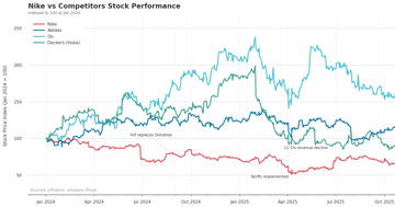
Nike's Crisis and the Economics of Brand Decay
Nike lost $28B by weakening product development, athlete partnerships, and marketing simultaneously. Data-driven analysis of how complementary assets collapse.
Analysis 8 min InvestingInvesting
Michael Burry's $379 Newsletter
Michael Burry launches Substack warning AI markets mirror 1999. His Nvidia-Cisco comparison, the GPU depreciation debate, and what hyperscalers need to justify capex.
Commentary 5 min InvestingInvesting![Is AI Really Eating the World? AGI, Networks, Value [2/2] — AGI predictions miss the point. Multiple competing models means price war. Value …](https://static.philippdubach.com/cdn-cgi/image/fit=crop,gravity=right,width=360,height=189,quality=80,format=auto/ograph/ograph-eatingtheworld2.jpg)
Is AI Really Eating the World? AGI, Networks, Value [2/2]
AGI predictions miss the point. Multiple competing models means price war. Value flows to applications, customer relationships, and vertical integrators.
Essay 7 min AIAI![Is AI Really Eating the World? [1/2] — Hyperscalers spend $400B on AI, API prices drop 97%, and DeepSeek builds …](https://static.philippdubach.com/cdn-cgi/image/fit=crop,gravity=right,width=360,height=189,quality=80,format=auto/ograph/ograph-eatingtheworld1.jpg)
Is AI Really Eating the World? [1/2]
Hyperscalers spend $400B on AI, API prices drop 97%, and DeepSeek builds frontier models for $500M. Value is flowing to applications, not model providers.
Analysis 5 min AIAI
Weather Forecasts Have Improved a Lot
Four-day forecasts now match one-day accuracy from 30 years ago. How AI models like WeatherNext 2 use CRPS training to preserve extreme weather signals.
Analysis 2 min AIAI
GLP-1 Receptor Agonists in ASUD Treatment
A phase 2 RCT shows low-dose semaglutide reduces alcohol craving and heavy drinking with effect sizes exceeding naltrexone. What GLP-1 means for AUD treatment.
Commentary 2 min MedicineMedicine
The Bicycle Needs Riding to be Understood
Build an LLM agent in 50 lines of Python. Why context engineering and emergent behaviors are best understood through hands-on experimentation, not theory.
Commentary 1 min AIAI
AI Models as Standalone P&Ls
OpenAI lost $11.5B in one quarter. But Anthropic CEO Dario Amodei argues each AI model is independently profitable. Here's why the math is complicated.
Commentary 4 min AIAI
Working with Models
Diffusion models corrupt data into noise, then reverse the process. Learn the math with Stefano Ermon's Stanford CS236 course, free on YouTube.
Commentary 1 min AIAI![Pozsar's Bretton Woods III: Three Years Later [2/2] — Gold above $4,000, Treasury holdings below $7T, but the dollar still dominates …](https://static.philippdubach.com/cdn-cgi/image/fit=crop,gravity=right,width=360,height=189,quality=80,format=auto/ograph/ograph-Pozsar2.jpg)
Pozsar's Bretton Woods III: Three Years Later [2/2]
Gold above $4,000, Treasury holdings below $7T, but the dollar still dominates 88% of FX volumes. What Pozsar's Bretton Woods III got right and wrong.
Analysis 6 min MacroMacro![Pozsar's Bretton Woods III: The Framework [1/2] — How freezing Russian reserves sparked Bretton Woods III: Pozsar's framework on …](https://static.philippdubach.com/cdn-cgi/image/fit=crop,gravity=right,width=360,height=189,quality=80,format=auto/ograph/ograph-Pozsar1.jpg)
Pozsar's Bretton Woods III: The Framework [1/2]
How freezing Russian reserves sparked Bretton Woods III: Pozsar's framework on inside money, outside money, and the shift to a commodity-backed monetary order.
Analysis 7 min MacroMacro
Everything is a DCF Model
Michael Mauboussin's argument that every cash-generating asset is valued through a DCF model. Why this Morgan Stanley paper changed how I think about value.
Commentary 1 min InvestingInvesting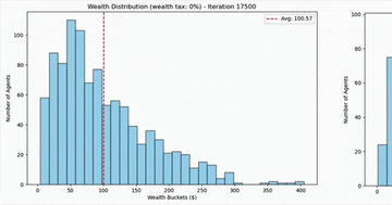
Agent-based Systems for Modeling Wealth Distribution
Agent-based modeling shows how random market transactions naturally produce extreme wealth concentration, and why even a small wealth tax changes everything.
Analysis 2 min EconomicsEconomics
Sentiment Trading Revisited
A Rutgers study finds news sentiment embeddings from OpenAI models cut stock price prediction errors by 40%. Time-independent models perform just as well.
Commentary 2 min AIAINovo Nordisk's Post-Patent Strategy
Amycretin's Phase 1 data shows 24.3% weight loss, beating Wegovy and Zepbound. How Novo Nordisk plans to replace its $20B Ozempic franchise before 2031.
Commentary 5 min MedicineMedicine
Behavioral Economics & Transit Policy
The zero price effect explains why politicians love free transit proposals. But making buses free might weaken the rider advocacy that protects service quality.
Analysis 4 min EconomicsEconomics
It Just Ain’t So
Are stock returns normally distributed? Formal normality tests reject this assumption for most equity indices, with major implications for risk management.
Commentary 2 min Quantitative FinanceQuant
Not All AI Skeptics Think Alike
Apple's Illusion of Thinking paper found AI reasoning models collapse at high complexity. But critics argue the methodology, not the models, may be flawed.
Commentary 2 min AIAIGambling vs. Investing
Kalshi's CFTC-regulated exchange now offers sports betting nationwide. If you can bet on oil futures, why not NFL touchdowns? The line is thinner than you think.
Commentary 2 min InvestingInvestingThe Model Said So
LLMs excel at parsing market sentiment and writing reports, but finance demands audit trails and explainable decisions that black box models cannot provide.
Commentary 1 min AIAIDual Mandate Tensions
New NBER paper shows optimal Fed policy should partially accommodate tariff inflation, exposing a fault line in the dual mandate when prices and jobs conflict.
Commentary 1 min MacroMacroBeyond Monte Carlo: Tensor-Based Market Modeling
UBS paper uses Transition Probability Tensors to bridge machine learning and arbitrage-free derivatives pricing, offering a faster alternative to Monte Carlo.
Commentary 2 min Quantitative FinanceQuantPassive Investing's Active Problem
Research shows passive investing makes markets more volatile as index fund growth amplifies each trade's price impact while active managers lag behind.
Commentary 2 min InvestingInvestingAlphaFold 3: Free for Science
Google released AlphaFold 3 for free, predicting molecular interactions beyond proteins. But is this generosity or a cloud platform play to own drug discovery?
Commentary 1 min MedicineMedicineAbout these essays
- What does Philipp Dubach write about?
- Long-form essays, analyses, and notes on quantitative finance, AI, and technology. Independent research-style writing — not commentary, not aggregation. Some essays are formalized as peer-reviewed papers and pre-prints with DOIs on SSRN and arXiv.
- How often are essays published?
- There is no fixed schedule. Essays appear when an idea is worth writing up, typically a few times a month. Subscribers receive new essays by email; the RSS and JSON feeds carry the same content.
- Where can I find the source code or papers behind these essays?
- Essays that ship with code link to public GitHub repositories inline. Peer-reviewed papers and pre-prints are listed on the Research page with DOI links to SSRN and arXiv. Builds and reproducible projects are catalogued on the Projects page.