Latest Posts

Earlier this year I wrote how I built a CGM data reader after wearing a continuous glucose monitor myself. Since I was already logging my macronutrients and learning more about molecular biology in an MIT MOOC I became curious if given a meal’s macronutrients (carbs, protein, fat) and some basic individual characteristics (age, BMI), these could serve as features in a regressor machine learning model to predict the curve parameters of the postprandial glucose curve (how my blood sugar levels change after eating). I came across a paper on Personalized Nutrition by Prediction of Glycemic Responses which did exactly that. Unfortunately, neither the data nor the code were publicly available. And - I wanted to predict my own glycemic response curve. So I decided to build my own model. In the process I wrote this working paper. 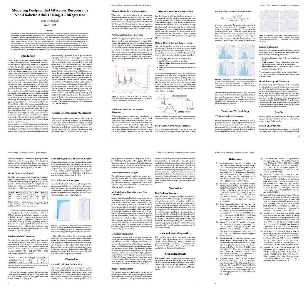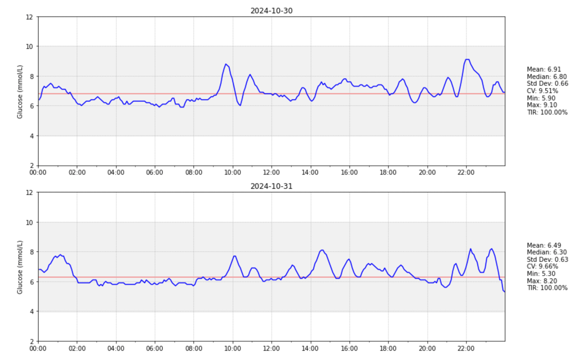The paper represents an exercise in applying machine learning techniques to medical applications. The methodologies employed were largely inspired by Zeevi et al.’s approach. I quickly realized that training a model on my own data only was not very promising if not impossible. To tackle this, I used the publicly available Hall dataset containing continuous glucose monitoring data from 57 adults, which I narrowed down to 112 standardized meals from 19 non-diabetic subjects with their respective glucose curve after the meal (full methodology in the paper). 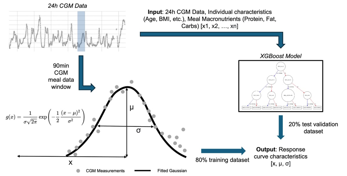Rather than trying to predict the entire glucose curve, I simplified the problem by fitting each postprandial response to a normalized Gaussian function. This gave me three key parameters to predict: amplitude (how high glucose rises), time-to-peak (when it peaks), and curve width (how long the response lasts). 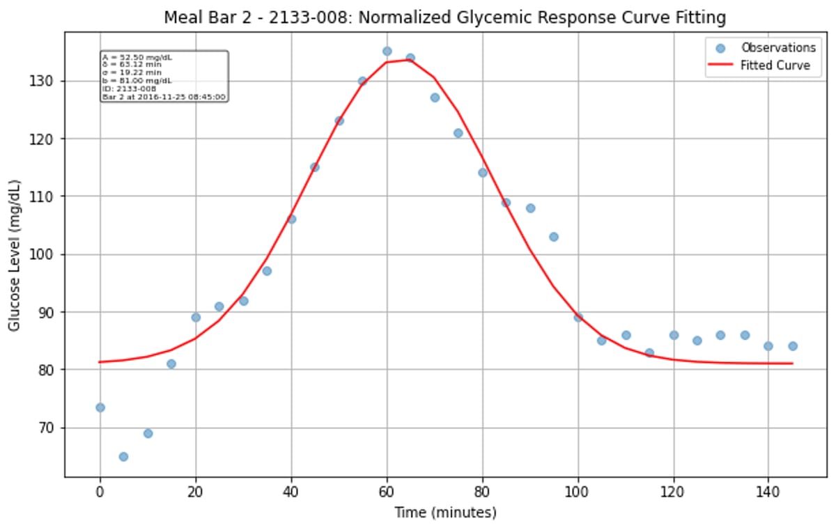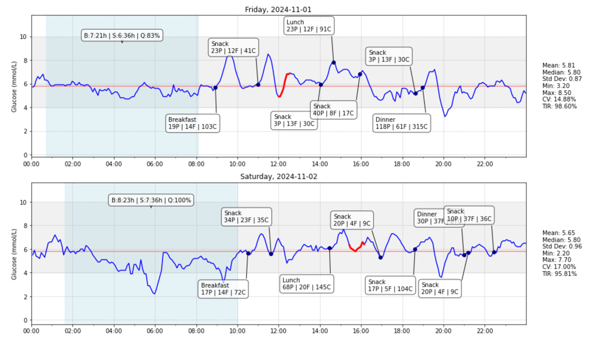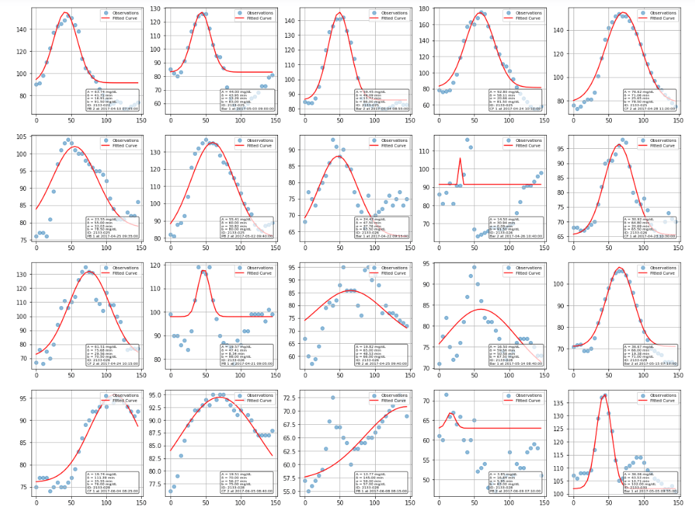The Gaussian approximation worked surprisingly well for characterizing most glucose responses. While some curves fit better than others, the majority of postprandial responses were well-captured, though there’s clear variation between individuals and meals. Some responses were high amplitude, narrow width, while others are more gradual and prolonged. I then trained an XGBoost regressor with 27 engineered features including meal composition, participant characteristics, and interaction terms. XGBoost was chosen for its ability to handle mixed data types, built-in feature importance, and strong performance on tabular data. The pipeline included hyperparameter tuning with 5-fold cross-validation to optimize learning rate, tree depth, and regularization parameters. Rather than relying solely on basic meal macronutrients, I engineered features across multiple categories and implemented CGM statistical features calculated over different time windows (24-hour and 4-hour periods), including time-in-range and glucose variability metrics. Architecture wise, I trained three separate XGBoost regressors - one for each Gaussian parameter.

While the model achieved moderate success predicting amplitude (R² = 0.46), it completely failed at predicting timing - time-to-peak prediction was essentially random (R² = -0.76), and curve width prediction was barely better (R² = 0.10). Even the amplitude prediction, while statistically significant, falls well short of an R² > 0.7. Studies that have achieved better predictive performance typically used much larger datasets (>1000 participants). For my original goal of predicting my own glycemic responses, this suggests that either individual-specific models trained on extensive personal data, or much more sophisticated approaches incorporating larger training datasets, would be necessary.

The complete code, Jupyter notebooks, processed datasets, and supplementary results are available in my GitHub repository.
_ _

(10/06/2025) Update: Today I came across Marcel Salathé’s LinkedIn post on a publication out of EPFL: Personalized glucose prediction using in situ data only.

With data from over 1,000 participants of the Food & You digital cohort, we show that a machine learning model using only food data from myFoodRepo and a glucose monitor can closely track real blood sugar responses to any meal (correlation of 0.71).

As expected Singh et. al. achieve a substantially better predictive performance (R = 0.71 vs R² = 0.46). Besides probably higher methodological rigor and scientific quality, the most critical difference is sample size - their 1'000+ participants versus my 19 participants (from the Hall dataset) represents a fundamental difference in statistical power and generalizability. They addressed one of the shortcomings I faced by leveraging a large digital nutritional cohort from the “Food & You” study (including high-resolution data of nutritional intake of more than 46 million kcal collected from 315'126 dishes over 23'335 participant days, 1'470'030 blood glucose measurements, 49'110 survey responses, and 1'024 samples for gut microbiota analysis).

Apart from that I am excited to - at a first glance - observe the following similarities: (1) Both aim to predict postprandial glycemic responses using machine learning, with a focus on personalized nutrition applications. (2) Both employ XGBoost regression as their primary predictive algorithm and use similar performance metrics (R², RMSE, MAE, Pearson correlation). (3) Both extract comprehensive feature sets including meal composition (macronutrients), temporal features, and individual characteristics. (4) Both use mathematical approaches to characterize glucose responses - I used Gaussian curve fitting, while Singh et. al. use incremental area under the curve (iAUC). (5) Both employ cross-validation techniques for model evaluation and hyperparameter tuning. (6) SHAP Analysis: Both use SHAP for model interpretability and feature importance analysis.

Kalshi, a prediction market startup, is using its federal financial license to offer sports betting nationwide, even in states where it’s not legal. The move has earned them cease-and-desist letters from state gaming regulators, but CEO Tarek Mansour isn’t backing down:

We can go one by one for every financial market and it would fall under the definition of gambling. So what’s the difference?

It’s a question that cuts to the heart of modern finance. The founders argue that Wall Street blurred the line between investing and gambling long ago, and casting Kalshi as the latter is inconsistent at best. They have a point—if you can bet on oil futures, Nvidia’s stock price, or interest rate movements, why is wagering on NFL touchdowns more objectionable?

Benefiting from the Trump administration’s hands-off regulatory approach, with the CFTC dropping its legal challenge to their election contracts, the odds might be in their favor. Even better, a Kalshi board member is awaiting confirmation to lead the very agency that was previously their biggest antagonist.

The technical distinction matters: Kalshi operates as an exchange between traders rather than a house taking bets against customers. But functionally, with 79% of their recent trading volume being sports-related, they’re forcing us to confront an uncomfortable reality about risk, speculation, and what we choose to call “investing.”

Whether you call it innovation or regulatory arbitrage, Kalshi is exposing the arbitrary nature of the lines we’ve drawn around acceptable financial speculation.
_ _

(17/06/2025) Update: Matt Levine - one of the finance columnists I enjoy reading most - just published a long piece “It’s Not Gambling, It’s Predicting” in his newsletter on exactly this issue:

Kalshi offers a prediction market where you can bet on sports. No! Sorry! Wrong! It offers a prediction market where you can predict which team will win a sports game, and if you predict correctly you make money, and if you predict incorrectly you lose money. Not “bet on sports.” “Predict sports outcomes for money.” Completely different.

LLMs make your life easier until they don’t.

Their intrinsic complexity and lack of transparency pose significant challenges, especially in the highly regulated financial sector

Unlike other industries where “the model said so” might suffice, finance demands audit trails, bias detection, and explainable decision-making—requirements that sit uncomfortably with neural networks containing billions of parameters. The research highlights a fundamental tension that’s about to reshape fintech: the same complexity that makes LLMs powerful at parsing market sentiment or generating investment reports also makes them regulatory nightmares in a sector where you need to explain every decision to examiners.

Something interesting just happened at the National Bureau of Economic Research NBER

We study the optimal monetary policy response to the imposition of tariffs in a model with imported intermediate inputs. In a simple open-economy framework, we show that a tariff maps exactly into a cost-push shock in the standard closed-economy New Keynesian model, shifting the Phillips curve upward. We then characterize optimal monetary policy, showing that it partially accommodates the shock to smooth the transition to a more distorted long-run equilibrium—at the cost of higher short-run inflation.

Here’s where it gets interesting for current policy: Werning et. al. show that “optimal” monetary policy would actually calls for partial accommodation of tariff shocks—essentially allowing some inflation to persist to smooth the transition to what they euphemistically call “a more distorted long-run equilibrium.” With core PCE still running above the Fed’s 2% target and renewed tariff threats on the horizon, this research suggests Powell may need to abandon his recent dovish pivot and prepare for rate hikes that prioritize price stability over employment concerns. The dual mandate was never meant to be dual when the two mandates point in opposite directions.

A fascinating new paper from Stefano Iabichino at UBS Investment Bank explores what happens when you take the attention mechanisms powering modern AI and apply them to Wall Street’s most fundamental pricing problems, tackling what might be quantitative finance’s most intractable challenge.

The problem is elegantly simple yet profound: machine learning models are great at finding patterns in historical data, but financial theory demands that arbitrage-free prices be independent of past information. As the authors put it:

We contend that a fundamental tension exists between the usage of ML methodologies in risk and pricing and the First Fundamental Theorem of Finance (FFTF). While ML models rely on historical data to identify recurring patterns, the FFTF posits that arbitrage-free market prices are independent of past information.

Their solution? Transition Probability Tensors (TPTs) that function like attention mechanisms in neural networks, dynamically weighting relationships between risk factors while maintaining mathematical rigor. Instead of learning from history, these tensors capture “dynamic, context-aware relationships across dimensions” in real-time.

The practical results are impressive: simulating 210 quantitative investment strategies across 100,000 market scenarios in just 70 seconds, while identifying optimal hedging strategies and stress-testing future market conditions. The framework even adapts to different volatility regimes, shifting focus toward tail events during high-volatility periods—exactly like attention mechanisms focusing on relevant context. Whether it scales beyond this impressive proof-of-concept remains to be seen, but it’s seems to be a genuine attempt to resolve the fundamental tension between AI’s pattern-seeking nature and finance’s requirement for arbitrage-free pricing.

A new academic review by Ali Farhani reveals that institutional Total Value Locked in DeFi protocols hit $42 billion in 2024, with BlackRock leading the charge by launching a $250 million tokenized fund on Centrifuge.

The numbers tell a remarkable story of maturation. Layer 2 solutions like Optimism and Arbitrum now dominate the scaling landscape, while zero-knowledge proofs have reduced compliance costs by 30%. Even the terminology is evolving—researchers now discuss “Total Value Redeemable” instead of the traditional TVL metric, acknowledging that not all locked value is immediately liquid. Despite technological advances, security incidents persist with painful regularity: $350 million lost in the Wormhole bridge exploit, $81 million in Orbit Chain’s multi-signature failure. Cross-chain bridges remain “high-risk attack targets,” a sobering reminder that connecting different blockchains is still more art than science. The regulatory landscape is complicated as well. Europe’s MiCA regulation provides clear frameworks, while the SEC maintains its enforcement-first approach. Hong Kong’s innovation sandbox offers a third path, balancing experimentation with oversight.

DeFi is transitioning from a disruptive experiment to an integrated component of the global financial system

That transition isn’t complete—Layer 2 solutions are projected to host over 70% of DeFi TVL by mid-2025—but the direction is clear.

This post is based in part on a 2022 presentation I gave for the ICBS Student Investment Fund and my seminar work at Imperial College London.

As we were looking for new investment strategies for our Macro Sentiment Trading team, OpenAI had just published their GPT-3.5 Model. After first experiments with the model, we asked ourselves: How would large language models like GPT-3.5 perform in predicting sentiment in financial markets, where the signal-to-noise ratio is notoriously low? And could they potentially even outperform industry benchmarks at interpreting market sentiment from news headlines? The idea wasn’t entirely new. Studies [2] [3] have shown that investor sentiment, extracted from news and social media, can forecast market movements. But most approaches rely on traditional NLP models or proprietary systems like RavenPack. With the recent advances in large language models, I wanted to test whether these more sophisticated models could provide a competitive edge in sentiment-based trading. Before looking at model selection, it’s worth understanding what makes trading on sentiment so challenging. News headlines present two fundamental problems that any robust system must address. First, headlines are inherently non-stationary. Unlike other data sources, news reflects the constantly shifting landscape of global events, political climates, economic trends, etc. A model trained on COVID-19 vaccine headlines from 2020 might struggle with geopolitical tensions in 2023. This temporal drift means algorithms must be adaptive to maintain relevance. Second, the relationship between headlines and market impact is far from obvious. Consider these actual headlines from November 2020: “Pfizer Vaccine Prevents 90% of COVID Infections” drove the S&P 500 up 1.85%, while “Pfizer Says Safety Milestone Achieved” barely moved the market at -0.05%. The same company, similar positive news, dramatically different market reactions.

When developing a sentiment-based trading system, you essentially have two conceptual approaches: forward-looking and backward-looking. Forward-looking models try to predict which news themes will drive markets, often working qualitatively by creating logical frameworks that capture market expectations. This approach is highly adaptable but requires deep domain knowledge and is time-consuming to maintain. Backward-looking models analyze historical data to understand which headlines have moved markets in the past, then look for similarities in current news. This approach can leverage large datasets and scale efficiently, but suffers from low signal-to-noise ratios and the challenge that past relationships may not hold in the future. For this project, I chose the backward-looking approach, primarily for its scalability and ability to work with existing datasets.

Rather than rely on traditional approaches like FinBERT (which only provides discrete positive/neutral/negative classifications), I decided to test OpenAI’s GPT-3.5 Turbo model. The key advantage was its ability to provide continuous sentiment scores from -1 to 1, giving much more nuanced signals for trading decisions. I used news headlines from the Dow Jones Newswire covering the 30 DJI companies from 2018-2022, filtering for quality sources like the Wall Street Journal and Bloomberg. After removing duplicates, this yielded 2,072 headlines. I then prompted GPT-3.5 to score sentiment with the instruction: Rate the sentiment of the following news headlines from -1 (very bad) to 1 (very good), with two decimal precision. To validate the approach, I compared GPT-3.5 scores against RavenPack—the industry’s leading commercial sentiment provider. The correlation was 0.59, indicating the models generally agreed on sentiment direction while providing different granularities of scoring. More interesting was comparing the distribution of the sentiment ratings between the two models. This could have been approximated closer through some fine tuning of the (minimal) prompt used earlier. I implemented a simple strategy: go long when sentiment hits the top 5% of scores, close positions at 25% profit (to reduce transaction costs), and maintain a fully invested portfolio with 1% commission per trade. The results were mixed but promising. Over the full 2018-2022 period, the GPT-3.5 strategy generated 41.02% returns compared to RavenPack’s 40.99%—essentially matching the industry benchmark. However, both underperformed a simple buy-and-hold approach (58.13%) during this generally bullish period. Relying on market sentiment when news flow is low can be a tricky strategy. As can be seen from the example of the Salesforce stock performance**,** the strategy remained uninvested over a large period of time due to a (sometimes long-lasting) negative sentiment signal. When I tested different timeframes, the sentiment strategy showed its strength during volatile periods. From 2020-2022, it outperformed buy-and-hold (22.83% vs 21.00%). As expected, sentiment-based approaches work better when markets are less directional and more driven by news flow. To evaluate whether the scores generated by our GPT prompt were more accurate than those from the RavenPack benchmark, I calculated returns for different holding windows. The scores generated by our GPT prompt perform significantly better in the short term (1 and 10 days) for positive sentiment and in the long term (90 days) for negative sentiment. (Note: For lower sentiment, negative returns are desirable since the stock would be shorted)

While the model performed well technically, this project highlighted several practical challenges. First, data accessibility remains a major hurdle—getting real-time, high-quality news feeds is expensive and often restricted. Second, the strategy worked better in a more volatile environment, which prompted many individual trades, creating substantial transaction costs that significantly impact returns. Perhaps most importantly, any real-world implementation would need to compete with high-frequency traders who can act on news within milliseconds. The few seconds required for GPT-3.5 to process headlines and generate sentiment scores are far from being competitive. Despite these challenges, the project demonstrated that LLMs can match industry benchmarks for sentiment analysis—and this was using a general-purpose model, not one specifically fine-tuned for financial applications. OpenAI (and others) today offer more powerful models at very low cost as well as fine-tuning capabilities that could further improve performance. The bigger opportunity might be in combining sentiment signals with other factors, using sentiment as one input in a more sophisticated trading system rather than the sole decision criterion. There’s also potential in expanding beyond simple long-only strategies to include short positions on negative sentiment, or developing “sentiment indices” that smooth out individual headline noise. Market sentiment strategies may not be optimal for long-term investing, but they show clear promise for shorter-term trading in volatile environments. As LLMs continue to improve and become more accessible, this might offer an opportunity to revisit this project.

(1) A new academic paper suggests the rise of passive investing may be fueling fragile market moves. (2) According to a study to be published in the American Economic Review, evidence is building that active managers are slow to scoop up stocks en masse when prices move away from their intrinsic worth. (3) Thanks to this lethargic trading behavior and the relentless boom in benchmark-tracking index funds, the impact of each trade on prices gets amplified, explaining how sell orders can induce broader equity gyrations

Passive investing, the supposedly boring strategy of buying and holding index funds, might actually be making markets more volatile. A new study set to be published in the American Economic Review finds that active managers are slow to scoop up stocks when prices move away from their intrinsic worth. Meanwhile, the relentless boom in benchmark-tracking index funds means that each trade gets amplified, explaining how sell orders can induce broader equity gyrations. Justina Lee for Bloomberg writes that this week’s AI-fueled market swings perfectly illustrate the phenomenon. Big equity gauges plunged on Monday over fears about an AI model, before swiftly rebounding.

Thanks to this lethargic trading behavior and the relentless boom in benchmark-tracking index funds, the impact of each trade on prices gets amplified.

The researchers from UCLA, Stockholm School of Economics, and University of Minnesota have identified what they call “Big Passive”—a financial landscape that’s proving less dynamic and more volatile. When most investors are on autopilot, the few remaining active traders have disproportionate influence. This doesn’t invalidate passive investing’s core benefits—lower costs and better long-term returns for most investors remain compelling. But it does suggest that our increasingly passive financial system has some unintended consequences.

If you’re reading this, you might also be interested in: Modeling Glycemic Response with XGBoost

Last year I put a Continuous Glucose Monitor (CGM) sensor, specifically the Abbott Freestyle Libre 3, on my left arm. Why? I wanted to optimize my nutrition for endurance cycling competitions. Where I live, the sensor is easy to get—without any medical prescription—and even easier to use. Unfortunately, Abbott’s FreeStyle LibreLink app is less than optimal (3,250 other people with an average rating of 2.9/5.0 seem to agree). In their defense, the web app LibreView does offer some nice reports which can be generated as PDFs—not very dynamic, but still something! What I had in mind was more in the fashion of the Ultrahuman M1 dashboard. Unfortunately, I wasn’t allowed to use my Libre sensor (EU firmware) with their app (yes, I spoke to customer service).

At that point, I wasn’t left with much enthusiasm, only a coin-sized sensor in my arm. The LibreView website fortunately lets you download most of your (own) data in a CSV report (there is also a reverse engineered API), which is nice. So that’s what I did: download the data, pd.read_csv() it into my notebook, calculate summary statistics, and plot the values. After some interpolation, I now had the same view as the LibreLink app (which I had rejected earlier) provided. Yet, this setup allowed me to do further analysis and visualizations by adding other datapoints (workouts, sleep, nutrition) I was also collecting at that time:

• Blood sugar from LibreView: Measurement timestamps + glucose values
• Nutrition from MacroFactor: Meal timestamps + macronutrients (carbs, protein, and fat)
• Sleep data from Sleep Cycle: Sleep start timestamp + time in bed + time asleep (+ sleep quality, which is a proprietary measure calculated by the app)
• Cardio workouts from Garmin: Workout start timestamp + workout duration
• Strength workouts from Hevy: Workout start timestamp + workout duration

After structuring those datapoints in a dataframe and normalizing timestamps, I was able to quickly highlight sleep (blue boxes with callouts for time in bed, time asleep, and sleep quality) and workouts (red traces on glucose measurements for strength workouts, green traces for cardio workouts) by plotting highlighted traces on top of the historic glucose trail for a set period. Furthermore, I was able to add annotations for nutrition events with the respective macronutrients.

I asked Claude to create some sample data and streamline the functions to reduce dependencies on the specific data sources I used. The resulting notebook is a comprehensive CGM data analysis tool that loads and processes glucose readings alongside lifestyle data (nutrition, workouts, and sleep), then creates an integrated dashboard for visualization. The code handles data preprocessing including interpolation of missing glucose values, timeline synchronization across different data sources, and statistical analysis with key metrics like time-in-range and coefficient of variation. The main output is a day-by-day dashboard that overlays workout periods, nutrition events, and sleep phases onto continuous glucose monitoring data, enabling users to identify patterns and correlations between lifestyle factors and blood sugar responses.

You can find the complete notebook as well as the sample data in my GitHub repository.

The difference between green finance that works and green finance that doesn’t work seems to be commitment: Using a Difference-in-Differences model analyzing 2013-2023 bond data, researchers found no significant correlation between green bond issuance and CO2 emissions after net-zero policies were adopted. That’s the disappointing part. On the upside: companies issuing only green bonds showed higher ESG ratings, lower CO2 emissions, and lower financing costs, achieving substantial environmental benefits and economic advantages. Meanwhile, entities issuing both conventional and green bonds showed no environmental benefits, raising concerns about potential greenwashing.

Those issuing only green bonds tend to have higher ESG ratings, lower CO2 emissions, and lower financing costs.

This could be called the commitment premium: Companies that go all-in on green finance see real results – both environmental and financial. Those trying to have it both ways? They’re essentially paying green bond premiums for conventional bond performance while fooling nobody about their environmental impact. What are the implications for investors? We should favor pure-play green issuers, and regulators need standards that discourage this mixed-portfolio greenwashing. The study suggests current carbon reduction policies haven’t created sufficient pressure on bond issuers, but perhaps the market is already creating its own incentives.