# My First 'Optimal' Portfolio **Author:** Philipp D. Dubach | **Published:** March 15, 2024 | **Updated:** February 23, 2026 **Categories:** Investing **Keywords:** Python portfolio optimization, efficient frontier, Modern Portfolio Theory, Sharpe ratio, out-of-sample testing ## Key Takeaways - Mean-variance optimization tripled the Sharpe ratio from 0.65 to 1.68 while cutting volatility from 14.4% to 5.6% at the same 9.4% return - Out-of-sample testing across the 2018 bear market and 2019 bull market showed consistent CVaR reduction and improved risk-adjusted returns - The project was published as an academic paper to fill the gap between established MPT theory and the lack of accessible open-source Python optimization tools at the time --- My introduction to quantitative portfolio optimization happened during my undergraduate years, inspired by Attilio Meucci's [Risk and Asset Allocation](https://link.springer.com/book/10.1007/978-3-540-27904-4) and the convex optimization [teachings of Diamond and Boyd at Stanford](https://web.stanford.edu/~boyd/teaching.html). With enthusiasm and perhaps more confidence than expertise, I created my first "optimal" portfolio. What struck me most was the disconnect between theory and accessibility. Modern Portfolio Theory had been established since 1990, yet the optimization tools remained largely locked behind proprietary software. >Nevertheless, only a few comprehensive software models are available publicly to use, study, or modify. We tackle this issue by engineering practical tools for asset allocation and implementing them in the Python programming language. This gap inspired what would eventually be published as: [A Python integration of practical asset allocation based on modern portfolio theory and its advancements](https://digitalcollection.zhaw.ch/handle/11475/24351). My approach centered on a simple philosophy: >The focus is to keep the tools simple enough for interested practitioners to understand the underlying theory yet provide adequate numerical solutions. Today, the landscape has evolved dramatically. Projects like [PyPortfolioOpt](https://github.com/robertmartin8/PyPortfolioOpt) and [Riskfolio-Lib](https://github.com/dcajasn/Riskfolio-Lib) have established themselves as sophisticated open-source alternatives, far surpassing my early efforts in both scope and sophistication. 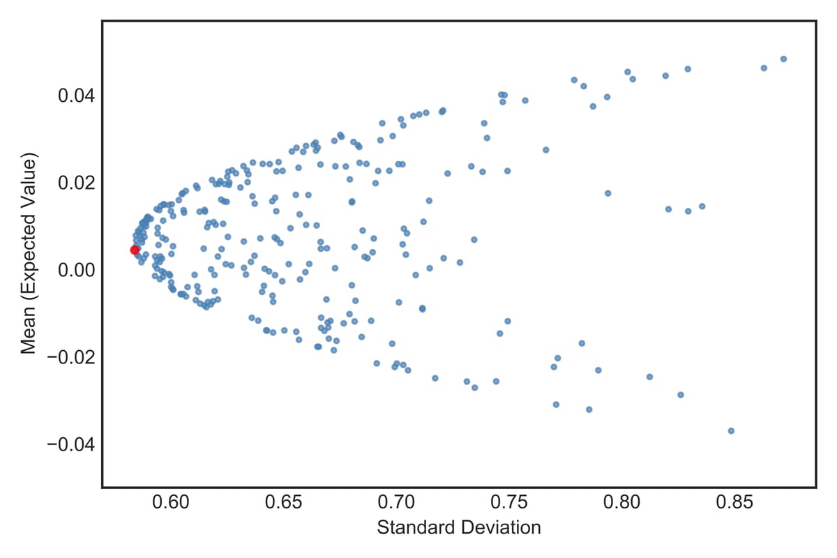Despite its limitations, the project yielded several meaningful insights: First, I set out to visualize Modern Portfolio Theory's fundamental principle—the risk-return tradeoff that drives optimization decisions. This scatter plot showing the efficient frontier demonstrates this core concept. 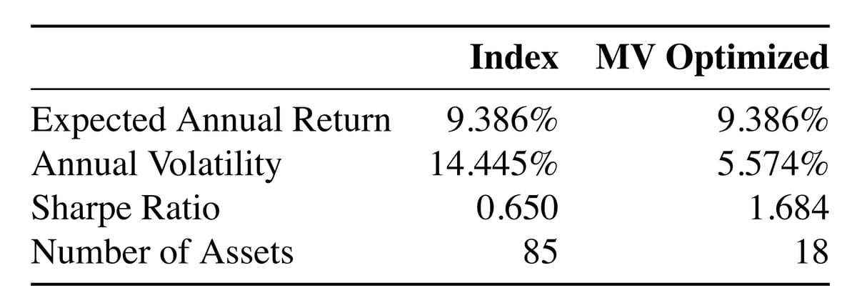The results of my first optimization: maintaining a 9.386% return while reducing volatility from 14.445% to 5.574%, effectively tripling the Sharpe ratio from 0.650 to 1.684. 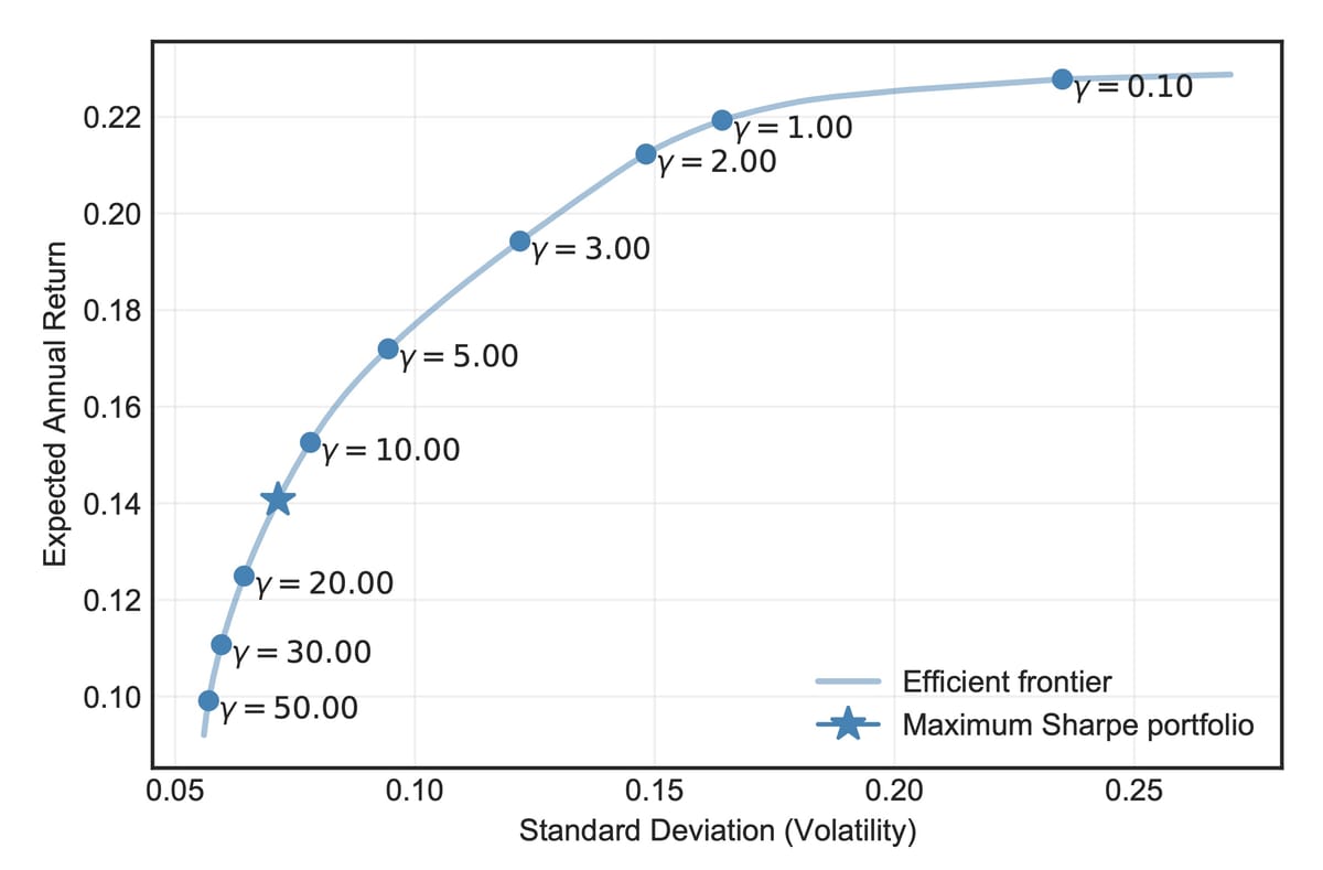By varying the risk aversion parameter (gamma), the framework successfully adapted to different investor profiles, demonstrating the flexibility of the optimization approach. This efficient frontier plot with different gamma values illustrates how the optimization framework adapts to different investor risk preferences. 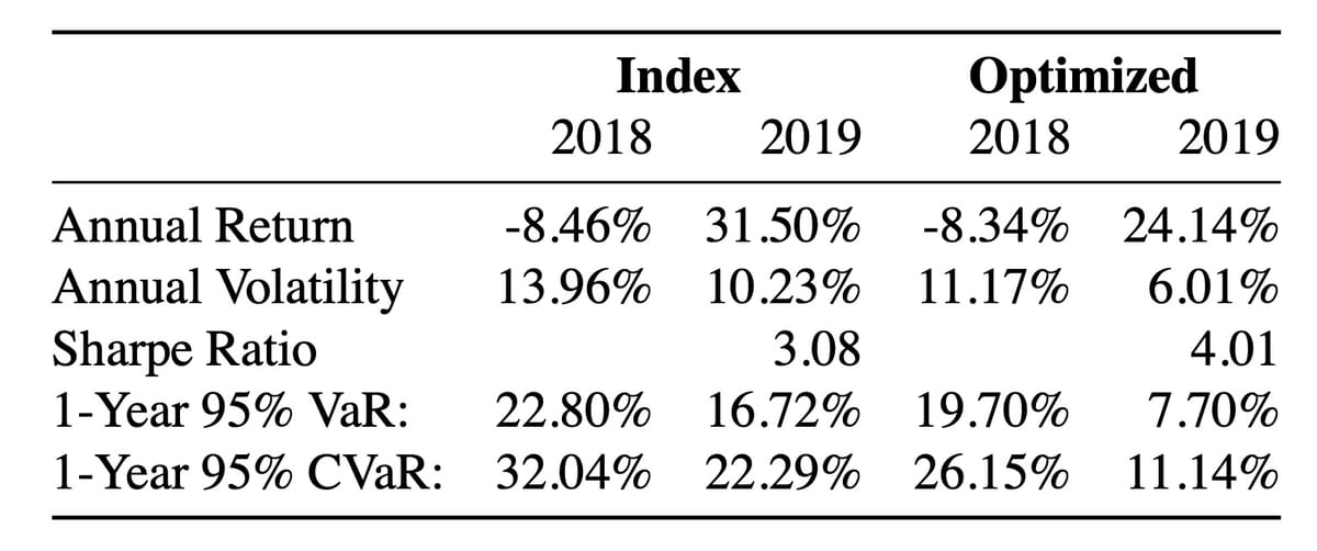Perhaps most importantly, out-of-sample testing across diverse market conditions—including the 2018 bear market and 2019 bull market—demonstrated consistent CVaR reduction and improved risk-adjusted returns. >We demonstrate how even in an environment with high correlation, achieving a competitive return with a lower expected shortfall and lower excess risk than the given benchmark over multiple periods is possible. Looking back, the project feels embarrassingly naive—and surprisingly foundational. While it earned some recognition at the time, it now serves as a valuable reminder: sometimes the best foundation is built before you know enough to doubt yourself. --- ## Frequently Asked Questions ### Can portfolio optimization actually improve the Sharpe ratio? Yes. In this project, applying mean-variance optimization to a multi-asset portfolio improved the Sharpe ratio from 0.650 to 1.684 while reducing volatility from 14.4% to 5.6%. The return was maintained at 9.4%. These results were validated through out-of-sample testing across both the 2018 bear market and 2019 bull market. ### How do you validate portfolio optimization with out-of-sample testing? Out-of-sample testing involves optimizing portfolio weights on historical data and then evaluating performance on a separate time period the model has never seen. This project tested optimized portfolios across diverse market conditions, demonstrating consistent CVaR reduction and improved risk-adjusted returns even in high-correlation environments. ### What Python libraries are available for portfolio optimization? The main open-source options today include PyPortfolioOpt (mean-variance, Black-Litterman, Hierarchical Risk Parity), Riskfolio-Lib (24 convex risk measures, Kelly Criterion optimization), and skfolio (built on scikit-learn). Before these libraries existed, practitioners had to build their own tools using SciPy and CVXPY, which is what motivated this project's original publication. ### What role does the risk aversion parameter play in portfolio optimization? The risk aversion parameter (gamma) controls how aggressively or conservatively the optimizer allocates assets. A higher gamma produces more conservative portfolios concentrated in lower-volatility assets, while a lower gamma allows the optimizer to take on more risk for higher expected returns. Varying gamma traces out different points along the efficient frontier, allowing the framework to adapt to different investor profiles. --- *Philipp D. Dubach — [http://philippdubach.com/](http://philippdubach.com/) — 2024*